Assessment of corrected time-step method for nominal ionospheric gradient calculation: A comparative analysis with spatial approaches

1.   Introduction

The ground-based augmentation system (GBAS) is a new aircraft landing assistance system using the global navigation satellite system (GNSS). The GNSS is susceptible to ionospheric delay, which can degrade the accuracy of the GBAS (International Civil Aviation Organization, 2016; Radio Technical Commission for Aeronautics, 2017a, b). The GBAS corrects range errors attributable to ionospheric delay by placing reference receivers around an airport to observe GNSS signals continuously. A difference in ionospheric delay will always exist as the separation distance between the runway and the aircraft increases. The difference in the ionospheric delay under normal conditions is often referred to as the nominal ionospheric gradient (σ_vig).

The magnitude of σ_vig is usually determined by spatial single-difference (SD) methods. Initially, spatial difference methods (mixed-pair and station-pair) were proposed to calculate σ_vig by using data from the Continuously Operating Reference Stations (CORS) Network in the observation area (Datta-Barua et al., 2002; Lee et al., 2006; Mayer et al., 2009). In the case of a nonideal CORS distribution, the satellite-pair method is more suitable. This method is built on the SD principle of two satellites at the same receiver (Supriadi et al., 2022).

Another method of estimating the value of σ_vig is carried out by using a temporal method known as the time step, which was first introduced by using Satellite-Based Augmentation System (SBAS) data (Datta-Barua et al., 2002). The SBAS is a geostationary satellite system used to transmit corrections and establish integrity for the global positioning system (GPS). It also provides pseudorange information. Because of its fixed position relative to the user in its footprint, the data obtained always pass through the same ionospheric pierce point (IPP).

A similar study was carried out later at maximum time intervals of 10 minutes (Lee et al., 2006). The time-step method uses the SD per epoch at a certain time interval per satellite so that it can eliminate the effects of satellite and receiver biases. The advantage of this method is its ability to calculate σ_vig when using only one receiver (a single receiver or a single station). However, the two studies mentioned showed that the magnitude of σ_vig was greater than with the spatial difference method (station-pair) because of the ionospheric temporal variation included therein.

The time-step method was then used to determine anomalous ionospheric gradients (Pradipta and Doherty, 2016). The use of the time-step method for σ_vig analysis was carried out in India by dividing its territory into three regions, which included low and mid-latitudes (Ammana and Achanta, 2016). The study used data from SBAS stations that were far from each other, and the number was limited, which made the time-step method quite suitable for this region. The results showed a significant difference between the low and mid-latitudes. The σ_vig at low latitudes was greater than that at mid-latitudes (up to 32°N in India) even in quiet ionospheric conditions. The closer σ_vig was to low latitudes, the greater the ionospheric temporal variation became. We assume ionospheric temporal variations may still influence such results.

The use of the time-step method on a single receiver in real time on a single-frequency GPS was carried out in the region of Thailand (Budtho et al., 2020). However, none of the studies mentioned have analyzed a time-step correction method to eliminate temporal variations.

It should be noted that the baseline of the time-step method is not omnidirectional but is limited by the satellite orbit. There are more north–south directions at low latitudes and more west–east directions at mid-latitudes. Note also that small-scale spatial fluctuations and their movement relative to the IPP could lead to uncertainty in the σ_vig estimation by the time-step method. The latter issue arises when using observational data, but not simulation data with an empirical ionospheric model, which is free from small-scale fluctuations.

The time-step method uses the SD of the two IPPs from one moving GNSS satellite. This results in the mixing of ionospheric spatial and temporal variations. To obtain the spatial variation in the ionospheric delay, we need to remove the temporal variation by first estimating the value as a correction. In this study, we propose a method to distinguish the spatial variations of the ionospheric delay from the temporal variations by using measurements from geostationary satellites as a correction. The method is tested with simulation data. The results of this study are not intended to replace the use of observational data from CORS, which have true σ_vig values.

2.   Data and Methodology

To estimate the temporal variation, we must measure the change at one fixed IPP. Global positioning system satellites are medium Earth orbit satellites that will always move. Geostationary satellites, on the other hand, have fixed orbits around the Earth that make them suitable for estimating temporal variations. The temporal variation is then applied to the time-step results as a correction to the spatial variation. The difference in total electron content between GPS and geostationary satellites is negligible because the electron density above GPS satellites is extremely small (Jakowski and Hoque, 2018). In addition, the σ_vig estimation is performed during quiet ionospheric conditions.

Testing the correction method by using observational data is difficult because the correction method test requires dual-frequency geostationary satellite data. These data are not acquired by the existing CORS. To address this difficulty, we use simulation data from the global ionospheric model (GIM) to test the correction value derived from the GIM to the time-step method derived from the GIM.

Our main data are generated from a simulation obtained from the IONosphere map EXchange (IONEX) file, which can be downloaded from the International GNSS Service (IGS) website. The IONEX file provides total electron content data, which can be derived from the ionospheric delay per grid with a size of 2.5° in the latitude direction and 5° in the longitude direction. Simulation data can be obtained by interpolating the ionospheric delay data within the grid. The simulated ionospheric delay is then compared with the observed ionospheric delay to see how closely the simulation represents the actual observation conditions. If the trend and the value of the ionospheric delay from both the simulation and observation are not too different, then the simulation data can be assumed to be used for testing. To do so, it is necessary to use the same time and location for validation.

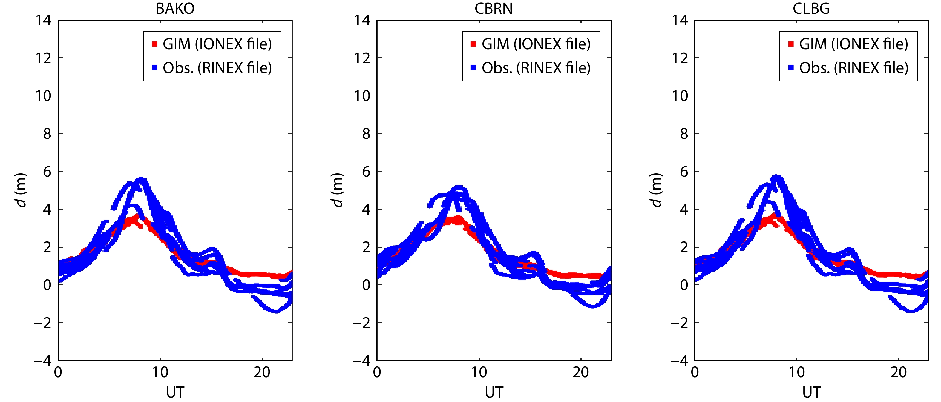
The main input for the simulation is the CORS location and time. Figure 1 shows a comparison between the observed (blue) and simulated (red) ionospheric delay at the CORS location at the BAKO site (106.84°E, 6.49°S), CBRN site (114.44°E, 7.83°S), and CLBG site (107.61°E, 6.82°S) on the same day (January 1, 2009) for reference stations 1 to 3. Observational data are generated from the GNSS measurement data in Receiver Independent Exchange (RINEX) format by using Long-Term Ionospheric Anomaly Monitor (LTIAM) software (Lee et al., 2011; Jung and Lee, 2012). The LTIAM software uses an interfrequency bias (IFB) estimation method that assumes the vertical ionospheric delay is identical within a 2° longitude by 2° latitude grid mesh (Ma and Maruyama, 2003). The simulation data are generated from the GIM data in IONEX format provided by the IGS (Schaer et al., 1998).

Figure  1.  Comparison of ionospheric delay between observations derived from the RINEX file (blue dots) and simulations derived from the GIM or IONEX file (red dots). d is ionospheric delay in meter ; UT is universal time.

DownLoad: Full-Size Img PowerPoint

Figure 1 shows the general similarity in values, but of course, the observational results show more active ionospheric conditions. The observation is more dynamic between different arcs of the ionospheric delay of each satellite. One arc shows continuous observations of ionospheric delay. After the satellite is no longer observed, it creates a new ionospheric delay arc. Overall, the trend in ionospheric delay from both simulations and observations shows that the GIM data represent the observation well. Note that the GIM data are solely used to determine the suitability of the time-step correction. However, only observational data are necessary for σ_vig value calculations.

The vertical ionospheric delay (VID) data obtained from GNSS observations or simulation data are differentiated between satellites (satellite-pair), between receivers (station-pair), or between epochs (time-step). The commonly used method is the station-pair method, which differentiates the data to obtain the vertical ionospheric gradient (VIG) from the same satellite, thus ensuring that the satellite IFB from both observations from two receivers will be the same (IFB^S1) while the first bias (IFB_R1) will differ from the second (IFB_R2):

The second method is the satellite-pair method, which takes the difference between the ionospheric delay of a pair of satellites observed by the same receiver (VID^S1 and VID^S2). In this method, the IFB_R1 is eliminated even though a difference between the first bias (IFB^S1) and the second bias (IFB^S2) still exists:

The third method (mixed-pair) takes the difference between the ionospheric delay in each IPP pair regardless of which receiver and satellite the IPP originated from. The result of the mixed-pair method is a combination of spatial methods from the station-pair, satellite-pair, and different satellite and receiver methods. However, this method does not include a temporal component, as does the time-step method.

The fourth method is the time-step method, which uses a dual-frequency receiver that can use data from one satellite that are then differentiated at different epochs. This method can eliminate satellite bias and receiver bias:

Figure 2 shows the σ_vig estimation methods based on observations by station-pair and satellite-pair.

Figure  2.  The existing method: station-pair method (red dashed line), satellite-pair method (blue dashed line), and uncorrected time-step method.

DownLoad: Full-Size Img PowerPoint

The calculation of σ_vig from the four methods described above is performed by computing the mean and standard deviation of the ionospheric gradient (VID) dataset for each method (Ammana and Achanta, 2016). The VIG is normalized by subtracting the mean and dividing it by the standard deviation. The normalized ionospheric gradient dataset is then divided into several bins, with the width of each bin (w) given as

where j is the number of bins, a is the minimum value of the ionospheric gradient in the dataset, and b is the maximum value of the ionospheric gradient in the dataset.

If the ionospheric gradient dataset contains N data points and N_i is the number of values in bin i, estimation of the probability density function (PDF) can be given as

When calculating integrity parameters in GBAS, a Gaussian distribution with a mean of zero is assumed. The experimental data distribution is then compared with a Gaussian distribution with a mean of zero and an observed standard deviation (σ_{vig_obs}). Because the experimental data distribution is not a perfect Gaussian distribution and is often accompanied by heavy tails, the σ_{vig_obs} is inflated by a factor of f so that the Gaussian distribution with the inflated standard deviation (σ_{vig_overbound}) bounds the tails. We increase f by a step of 0.1 until the tails are bounded. Thus, σ_{vig_overbound} is given as

Furthermore, the gradients are divided into bins of the IPP distance difference on the x-axis and the ionospheric delay difference on the x-axis. The mean (μ_{vig_obs}) and standard deviation (σ_{vig_obs}) of the gradients in each bin are evaluated and used in estimating σ_{vig_overbound} as described in Equation (5).

The PDF of VIG events is obtained from the VIG value calculated by Equation (5). The normal distribution represented by the standard deviation value cannot cover all the observed PDFs. Therefore, an inflation factor is needed that will be multiplied by the standard deviation so that the normal distribution with an increased standard deviation can include the PDF. The overbound standard deviation is called σ_vig.

The next stage focuses more on the use of the time-step correction method. The correction method test requires ideal conditions (a truth without noise) derived from the GIM. All the configurations needed for the simulation are obtained from the observational configurations. The configuration includes the CORS location, satellite position, and IPP. Figure 3 illustrates the method of development of the correction. An ionospheric delay from geostationary equatorial orbit (GEO) satellites, such as dual-frequency SBAS satellites, can produce temporal variations because the IPP is fixed to one location. This temporal variation is used for the area within a radius of 250 km from the central IPP of the SBAS satellite. This radius is equal to the elevation angle of 30° of a GPS satellite.

Figure  3.  Correction mechanism of the time-step method by using a fixed IPP location from a geostationary satellite viewed from the side (a) and from the top (b).

DownLoad: Full-Size Img PowerPoint

Extracting the ionospheric delay from geostationary satellite observations is not possible with the current CORS network capacity in Indonesia. The Indonesia Geospatial Information Agency (Badan Informasi Geospasial, BIG) provides only GPS and Russian GLObal NAvigation Satellite System (GLONASS) data, to keep the memory size of CORS data as small as possible. However, when using a simulation, this is possible by calculating the delay of the ionosphere at a fixed elevation angle of 90°. The magnitude of this temporal variation becomes a correction for the time-step method. Equation (3) will become

where ${\mathrm{V}\mathrm{I}\mathrm{D}}_{T2}^{{S}_{1}}$ is the ionospheric delay of satellite S₁ in epoch T₂ and ${\mathrm{V}\mathrm{I}\mathrm{D}}_{T1}^{{S}_{1}}$ is the ionospheric delay of satellite S₁ in epoch T₁. The difference between these two values divided by the IPP distance (R₁₂) is known by the uncorrected time-step method. The correction is built by adding the differences between the two geostationary satellite epochs ${(\mathrm{V}\mathrm{I}\mathrm{D}}_{T2}^{\mathrm{S}\mathrm{B}\mathrm{A}\mathrm{S}}-{\mathrm{V}\mathrm{I}\mathrm{D}}_{T1}^{\mathrm{S}\mathrm{B}\mathrm{A}\mathrm{S}})$. This value is used as the value of the temporal variation approach.

This correction assumes that in certain coverage areas, the temporal variations will be almost the same. This assumption limits the correction to only certain coverage, which, in this study, is limited to <5° longitude or latitude or equivalent to the satellites with an elevation mask of 30°. Moreover, an important point to consider is that the corrected time-step method is applicable only to a receiver that has not only the GPS measurement but also the dual-frequency SBAS enabled.

To assess the effectiveness of this method, we compare the results of the simulation and the observation. This comparison is relevant only when the configuration between the simulation and observation remains consistent. We use the same CORS configuration (the same location of CORS and the same satellite position) as for the simulation from previous research (Supriadi et al., 2022). For example, 66 CORS stations were used in the previous study for January 1, 2012. We use the positions of the 66 CORS stations as inputs for this simulation, as shown in Figure 4. The same CORS configuration on different days from previous research is also applied for the simulation.

Figure  4.  The methodology of the study regarding which CORS location data and RINEX navigation data are used as inputs to generate ionosphere delay data through the interpolation method of GIM data.

DownLoad: Full-Size Img PowerPoint

In addition to position information, satellite ephemeris data obtained from CORS are utilized to calculate the satellite positions. These two pieces of information, the CORS locations and the satellite positions, are used to calculate the IPP so that the ionospheric delay can be generated from the IONEX file by the interpolation method. The comparison between the ionospheric delay from IONEX data and observations is shown in Figure 1.

3.   Results

All the spatial difference methods, such as mixed-pair, station-pair, and satellite-pair, require a large number of receivers to calculate σ_vig. In contrast, the time-step method requires only one receiver. However, we need to study its limitations and avoid the effect of temporal variations. The temporal variation correction is developed from the fixed point of one IPP obtained from the ionospheric delay from a GEO satellite measurement.

The temporal variation at a specific IPP point is estimated to have the same value as the surrounding area up to a certain range. This range will be further detailed later on.

3.1   Time-Step Corrections from GIM

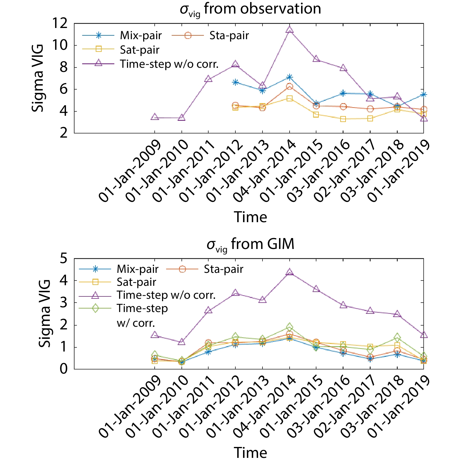
The top panel in Figure 5 shows the results of σ_vig when using the observational data from InaCORS from previous papers (Supriadi et al., 2022). The x-axis indicates every first quiet day (Kp index < 3) at the beginning of every year from 2009 to 2019, whereas the bottom panel in Figure 5 shows the new results from the simulation described in Section 2. The results of the spatial difference method cannot be applied to 3 days in the first 3 years (January 1, 2009; January 1, 2010; and January 1, 2011) because the number of CORS stations in the Indonesia area is insufficient and the distribution of the stations is inadequate during these 3 days. However, the time-step method is capable of calculating all available data because it can be used with just one receiver.

Figure  5.  Comparison between the time-step method and the spatial difference methods when using observational data (top) and simulation data (bottom).

DownLoad: Full-Size Img PowerPoint

The double-difference (DD) per epoch method within the time-step method makes the number of observations quite large, namely by differentiating the first epoch from the second epoch, then the first epoch from the third epoch, and so on as long as the difference between epochs is less than 10 minutes. However, the DD method between epochs in the time step will induce temporal variations because it subtracts two different epochs. The σ_vig results from the time-step method, which still contain temporal variations, have a greater value than the spatial difference method, as shown in Figure 5. However, the uncorrected time-step σ_vig, as shown in Figure 4, has a larger value than the spatial difference method.

Observations of fixed ionospheric delay at one IPP are difficult to obtain because dual-frequency data from the SBAS GEOs are not available in Indonesia. The validation process of the correction is feasible only when simulation data are used. The data generated in the simulation use the same CORS configuration as in the previous article (Supriadi et al., 2022). For instance, the blue color (mixed pair) in the lower panel of Figure 5 uses the same data source (CORS) and configuration as the blue color in the top panel of Figure 5. The configuration includes the CORS location and the same satellite constellation. Accordingly, the locations of CORS in 2012 are used as inputs to build a simulated ionospheric delay from the GIM at the observed IPP data.

From the ionospheric delay difference dataset, the parameter σ_vig is extracted. Distinct outcomes emerge between σ_vig from observations and simulations. The σ_vig value from the mixed pair (blue) using observational data is the largest, whereas when using the simulation, it becomes the smallest value among all the spatial difference methods. When using observational data, mixed-pair methods will include satellite and receiver bias, which makes the σ_vig value larger than with the station-pair (yellow) and satellite-pair methods (red). However, in the simulation, there is no satellite or receiver bias. Notably, within the simulation framework, the most reliable σ_vig is ascribed to the mixed-pair methods, primarily because of the substantial amount of data. The station-pair method contains a greater amount of data in comparison with the satellite-pair method.

The time-step method is constructed with the same satellite constellation but uses only a single receiver. The DD in the time-step method will cancel out the receiver and satellite bias. Figure 5 (top panel) shows a larger σ_vig of uncorrected time-step methods value than with the spatial difference methods. The potential candidates of this large value is the temporal variation. This is one of the weaknesses of the time-step method.

The σ_vig value using the uncorrected time-step method (purple) in the observations and simulations has a large correlation of 0.95 despite the big difference between both σ_vig values. Figure 5 (bottom panel) shows that σ_vig using the corrected time-step method (green) is closer to the spatial difference methods that use multiple receivers than to the uncorrected time-step method.

The correlation values between observation and simulation for all spatial difference methods are quite large (mixed-pair = 0.841, station-pair = 0.837, and satellite-pair = 0.816). The correlation value with station-pair is greater than that with satellite-pair because the IPP distances in the satellite-pair have larger values than the others.

3.2   Satellite Path Effect

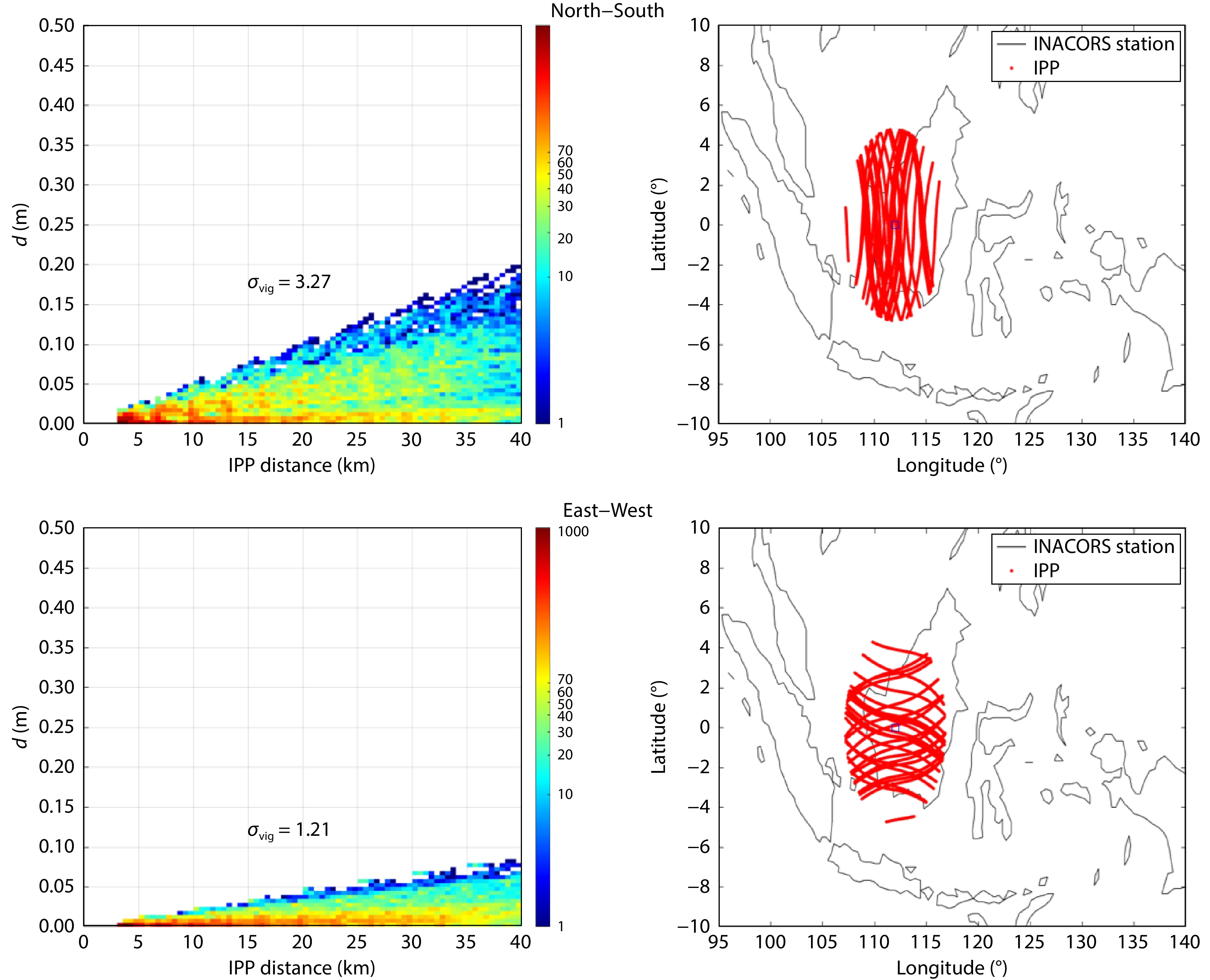
Another issue with using the time-step method at the equator is the direction of the satellite trajectory, which is not omnidirectional. As shown in Figure 6, the satellite path at the equator is more north–south. Ideally, the ionospheric gradient is constructed from different IPP pairs, both north–south and east–west, in contrast to the spatial difference method, which has an omnidirectional IPP pair because it uses all existing IPPs.

Figure  6.  Comparison of σ_vig from the normal satellite path, which tends toward the north–south direction in the region of the equator (top), and its rotation (90° to east) or the east–west direction (bottom) on January 4, 2014.

DownLoad: Full-Size Img PowerPoint

To address this difference, we rotate the satellite trajectory so that it is more west–east. The rotation center point is the location of the receiver. This process is possible only if we use IONEX data. The ionospheric delay data are generated by the east–west satellite path and then processed as in the previous step to produce the σ_vig value. The results in Figure 6 illustrate that the σ_vig value on the same day (January 4, 2014) in the east–west direction has a smaller value than that in the north–south direction. Therefore, applying the time-step method at the equator could cover the largest possible gradient so that integrity is maintained.

3.3   Coverage of the Correction

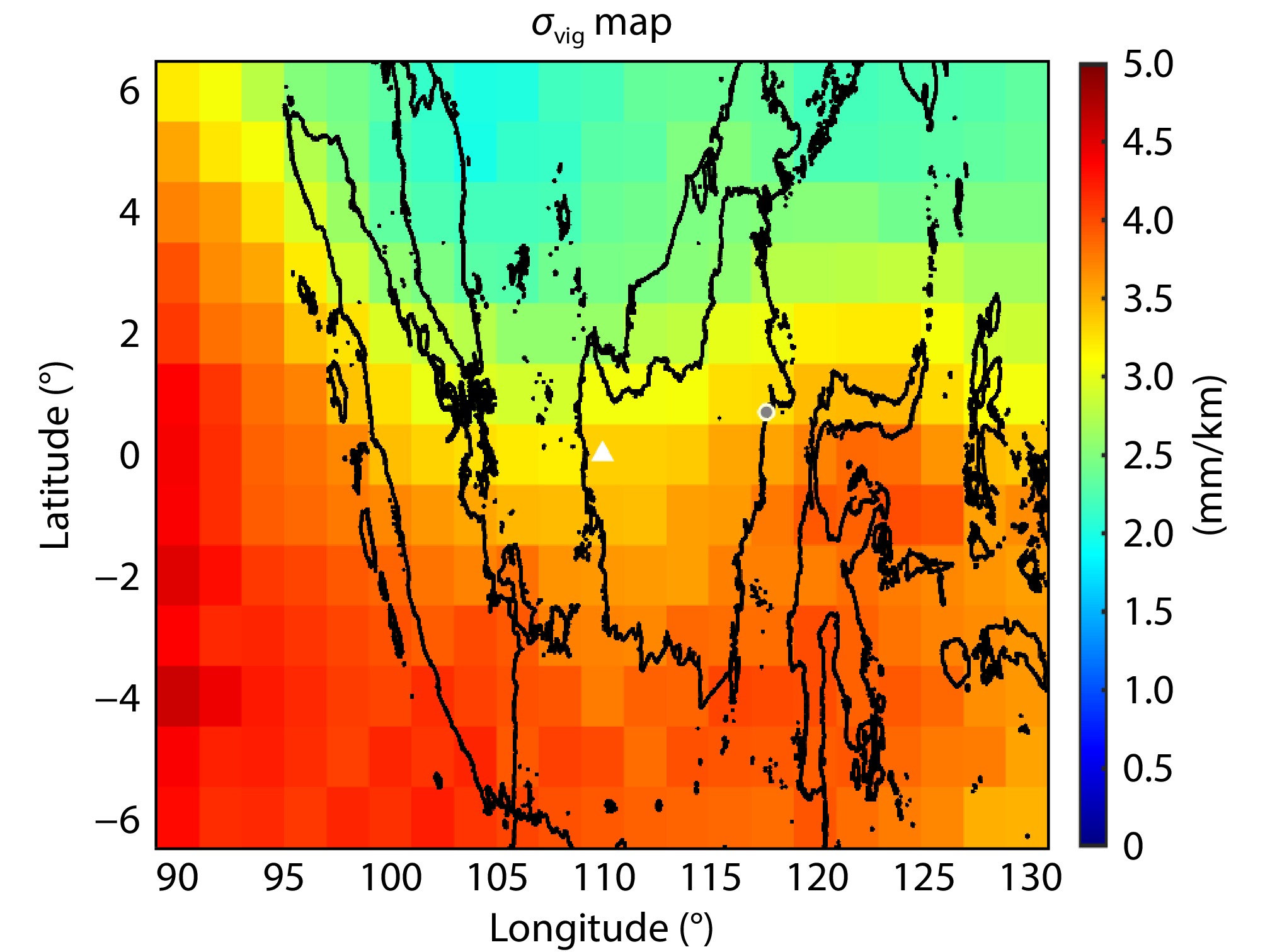
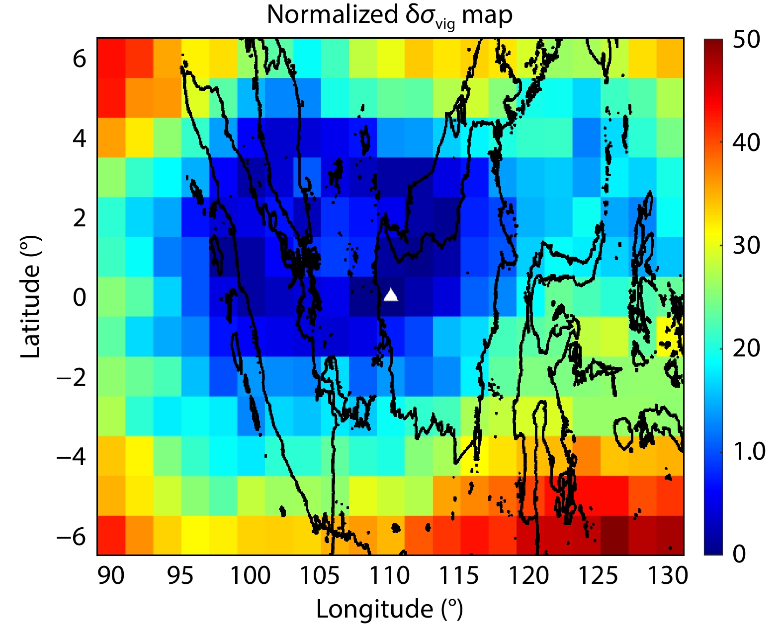
The coverage limit of the temporal variation correction for the time-step method must also be sought. To determine the limitations of the time-step correction method, we conduct two case studies. The first case study involves applying temporal corrections that are generated by using one SBAS receiver (110°E, 0°S) and applying them to other receivers in the surrounding area, at longitudes from 90°E to 130°E and latitudes from 6°S to 6°N, with a 1° step in longitude and a 2° step in latitude. The distance between the simulated SBAS receiver and the other receivers is 1° in latitude and 2° in longitude. In total, 273 receivers are simulated. Figure 7 shows the results of σ_vig for this first case, calculated by using the time-step method and corrections from the SBAS receiver (110°E, 0°S) with an SBAS satellite at the same longitude (i.e., at the zenith of the SBAS receiver). The white triangle represents the location of the reference point where temporal corrections are used for the grid of other receivers.

Figure  7.  The σ_vig value after applying the temporal variation correction from one reference point (110°E, 0°S), indicated by the white triangle.

DownLoad: Full-Size Img PowerPoint

The results shown in Figure 7 reveal significant differences, with σ_vig being larger in the southern region, likely because the region corresponds to the peak of the southern equatorial anomaly crest. Consequently, when the time-step correction is inaccurately applied in this area, the values tend to be higher compared with those in the northern region.

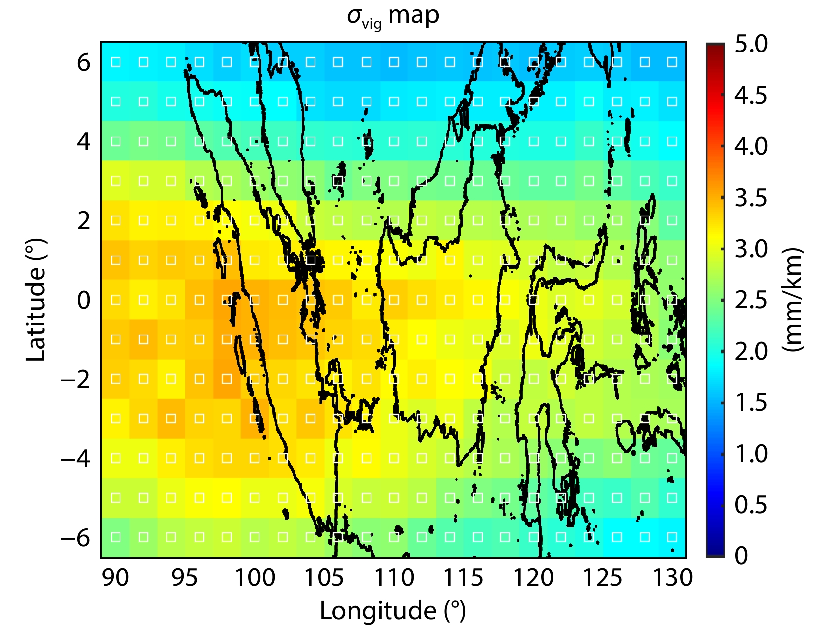
Next, we construct the second case study by using the time-step method corrected by the temporal variation of the ionospheric delay at the zenith of each receiver point, which is obtained from the GIM. Figure 8 shows the second case study, where the white squares indicate the locations of each point used as temporal variation correctors at those points. The results represent the corrected σ_vig values at their respective locations, as they should be. This second case is assumed to represent the true sigma values because it uses the correct temporal variation corrections and not their errors.

Figure  8.  The σ_vig value after applying the temporal variation correction from each grid.

DownLoad: Full-Size Img PowerPoint

The high value, around (100°, 0°), shows the high value of σ_vig in a day and not the error. Figure 8 illustrates the distribution of corrected σ_vig values when using GEO corrections at every location in the grid as the receiver observing GNSS measurements. Thus, Figure 8 serves as the reference σ_vig value for Figure 7. The satellite-pair and station-pair methods are indeed free from temporal variations, but the satellite-pair method is not free from satellite bias, and the station-pair method is not free from receiver bias. The satellite-pair method also produces only a high IPP distance, as shown in our previous study (Supriadi et al., 2022).

Figure 9 shows the normalized difference between the results of the first case study and the second case study. This difference indicates the error in using temporal variation corrections at a distant SBAS receiver. In other words, it demonstrates the limitations of using temporal variation corrections. The 0% error value is present only at the reference point (100°, 0°). Error values smaller than 5% are found in areas of 1° in latitude and 2° in longitude from the reference point. Error values smaller than 10% are found in areas of 2° in latitude and 4° in longitude from the reference point. The larger the distance from the reference point, the larger the error becomes.

Figure  9.  Normalized δσ_vig as the difference between applying the correction from only one reference point at (100°, 0°) and applying the correction from each grid location.

DownLoad: Full-Size Img PowerPoint

Temporal variation correction errors are more effective in the longitudinal direction compared with the latitudinal direction. This difference can be attributed to the fact that ionospheric variations exhibit a stronger latitudinal than longitudinal bias. Furthermore, the magnitudes of these correction errors are not uniform on the right and left sides of the reference point. The coverage area is also relatively limited, even though it is utilized for IONEX data, which is inherently less variable. This issue underscores the importance of using temporal variation corrections generated from the respective receiver for optimal results.

4.   Conclusions

In this study, we examine corrected time-step methods for calculating σ_vig and comparing the results with spatial difference methods, such as the mixed-pair, station-pair, and satellite-pair methods. Spatial difference methods require a substantial number of receivers for σ_vig calculations, whereas the time-step method stands out because it uses only a single receiver. Nontheless, it is crucial to understand the limitations of the time-step method and to address the effect of temporal variations.

Temporal variation corrections are developed based on fixed IPPs obtained from ionospheric delay measurements from geostationary satellites. These corrections are assumed to have similar values within a certain range of the surrounding IPPs. Hence, it is essential to acknowledge and address this range limitation.

The results indicate that despite the benefits of the time-step method, it introduces temporal variations because of the differential delay in different epochs, leading to higher σ_vig values compared with spatial difference methods. The uncorrected time-step method exhibits even larger σ_vig values than does the spatial difference methods.

Furthermore, the study highlights the challenges of obtaining observations of fixed ionospheric delays at one IPP because of the unavailability of dual-frequency data from SBAS in Indonesia. Therefore, validation of the correction method is feasible only through simulation data based on GIM maps, which demonstrates discrepancies between σ_vig values obtained from observations and simulations.

The study also addresses the issue of the satellite path direction at the equator, where satellite trajectories predominantly follow a north–south orientation. By rotating the satellite trajectory toward a west–east direction using IONEX data, we find that the σ_vig values decrease, in alignment with the expectation that zonal gradients will be smaller than meridional gradients.

Additionally, we explore the coverage limit of the temporal variation correction. Two case studies are conducted to evaluate the effectiveness of temporal corrections in different regions. The first case applies temporal corrections from a reference SBAS receiver to other receivers within a specific range and reveals significant differences in σ_vig values. The second case involves temporal corrections at each receiver point and is considered as representing the true σ_vig values. The optimal result is obtained when using temporal variation corrections generated from the respective receiver. In summary, the time-step method offers advantages in terms of data requirements, but its limitations related to temporal variations and coverage must be carefully considered.