Influence of annual atmospheric tide asymmetry on annual anomalies of the ionospheric mean state

1.   Introduction

In ionospheric studies, the term "anomaly" usually refers to an inconsistency between the electron density distribution observed in the F₂ layer and the result of the Chapman theory of photoionization. The ionospheric seasonal variabilities, which are important "ionospheric anomalies", is an unresolved important question in ionospheric research. Some previous studies have focused on the differences between summer and winter and between solstice and equinox (e.g., Zhao B et al., 2007); other research has focused on the asymmetry of the ionospheric seasonal variabilities. An interesting asymmetry in the ionospheric seasonal variation is the ionospheric annual anomaly (or ionospheric annual asymmetry). The ionospheric annual anomaly is characterized by the fact that the globally-averaged electron density is more than 20% larger in the December solstice than in the June solstice (e.g., Rishbeth and Müller-Wodarg, 2006). This difference has been observed in a series of ionospheric parameters, such as total electron content (TEC), F-layer peak electron density (N_mF₂), topside ionospheric electron density, and ionospheric electron density profiles (e.g. Su YZ et al., 1998; Mendillo et al., 2005; Rishbeth and Müller-Wodarg, 2006; Liu LB et al., 2007; Zeng Z et al., 2008; Sai Gowtam and Tulasi Ram, 2017).

The ionospheric annual anomaly’s physical mechanism has been listed as one of the top scientific objectives in ionosphere–thermosphere studies (Rishbeth, 2007). Using the CTIP (Coupled Thermosphere–Ionosphere–Plasmasphere) model, Rishbeth and Müller-Wodarg (2006) simulated the anomaly in the ionospheric peak electron density (N_mF₂), and found that the asymmetry of the Sun–Earth distance between the June and December solstices can partly explain the observed ionospheric annual anomaly. However, their simulated electron density anomaly was much smaller than the observed difference. Liu LB et al. (2007) studied the annual anomaly in the topside ionospheric total ion density at the height of 840 km, and pointed out that the observed anomaly can be partially explained by the annual asymmetry of the atomic oxygen density at that topside ionospheric height. Using the Thermosphere–Ionosphere Electrodynamics Global Circulation Model (TIEGCM), Zeng Z et al. (2008) simulated the ionospheric annual anomaly in N_mF₂, and successfully reproduced the observed N_mF₂ asymmetry. Their simulation suggested that the geomagnetic field configuration and the asymmetry of the Sun–Earth distance between the the June and December solstices are two primary processes that cause the ionospheric annual anomaly. However, why the 7% variance in the Sun–Earth distance should cause an asymmetry in ionospheric electron densities of more than 20% is still unknown. Mikhailov and Perrone (2011, 2015) suggested that a 7% increase in the O₂ dissociation rate associated with the June-to-December difference in the Sun–Earth distance is sufficient to explain the observed 21% annual anomaly in N_mF₂. However, using the Global Mean Model (Roble et al., 1987; Roble, 1995), Lei JH et al. (2016) simulated the annual O₂ dissociation asymmetry and found that the difference in solar EUV flux cannot explain the annual asymmetry in N_mF₂, and suggested, therefore, that the O₂ dissociation and atomic oxygen production mechanism are not the major drivers of the ionospheric annual anomaly. Using the TIEGCM, Dang T et al. (2017) simulated the influence on the annual ionospheric N_mF₂ anomaly of the June-to-December change in the Sun–Earth distance, and found that the distance change affects photochemical processes, thermospheric composition, and ionospheric diffusion.

Atmospheric tide can affect the coupled ionosphere–thermosphere system. Forbes et al. (1993) utilized the NCAR TIGCM to simulate tidal influences on the ionosphere and the thermosphere, and found that the upward propagating migrating tide can accelerate, heat, and mix the composition of the coupled ionosphere–thermosphere system. Jones et al. (2014) simulated impacts of vertically propagating tides on the mean state of the ionosphere and thermosphere, and found that the non-migrating tide DE3 also can affect the ionospheric mean state. Ren ZP et al. (2014) simulated the ionospheric influence of the DE3 tide, and found that it affects the equinoctial asymmetry of the zonal mean ionospheric electron density. Because the intra-annual variation of the atmospheric tide shows obvious annual asymmetry, the atmospheric tide may also affect the annual anomaly of the ionospheric mean states. The migrating diurnal and semi-diurnal tides both show obvious annual asymmetry, and may affect the ionospheric annual anomaly (see Forbes et al. (1993, 2008), Mukhtarov and Pancheva (2009) and Jones et al. (2014)). However, because the propagation and interactions between different tides are nonlinear, tidal influences on the ionospheric annual anomaly are very complex. Hence, in this paper, we will investigate mainly the atmospheric tide, using the GCITEM-IGGCAS and TIME3D-IGGCAS models to simulate its influence on the annual anomaly of the ionospheric zonal mean states.

2.   Model Descriptions and Inputs

To simulate the highly coupled and complex chemical and physical processes in the coupled ionosphere-thermosphere system, the Global Coupled Ionosphere–Thermosphere–Electrodynamics Model, Institute of Geology and Geophysics, Chinese Academy of Sciences (GCITEM-IGGCAS) has been developed. The GCITEM-IGGCAS is a three-dimensional (3-D) code with 5° latitude by 7.5° longitude cells in a spherical geographical coordinate system, based on an altitude grid. This model self-consistently calculates time-dependent 3-D structures of the main thermospheric and ionospheric parameters in the height range from 90 to 600 km, including neutral number density of major species O₂, N₂, and O and minor species N(²D), N(⁴S), NO, He and H; ion number densities of O⁺,O₂⁺, N₂⁺, NO⁺, N⁺ and electrons; neutral, electron and ion temperature; 3-D neutral winds; and ionospheric electric field. The GCITEM-IGGCAS can reproduce the main features of the coupled thermosphere and ionosphere system (see Ren ZP et al., 2009 for details).

Because of the spherical geographical coordinate system used in it, GCITEM-IGGCAS cannot self-consistently calculate the heat flux and plasma flux at the upper boundary, so we have had to obtain these fluxes from an empirical model. The TIME3D-IGGCAS is a three-dimension theoretical ionospheric model (Ren ZP et al., 2012a, b) that cover the whole ionosphere and the whole plasmasphere, and can self-consistently calculate the time-dependent three-dimensional structures of their main parameters in realistic geomagnetic fields, including electron and main ion (O⁺, H⁺, He⁺, NO⁺, O₂⁺, N₂⁺) number densities; electron and ion temperatures; and field-aligned ion velocities.

The TIME3D-IGGCAS and GCITEM-IGGCAS models can two-way couple with each other. In this condition, the GCITEM-IGGCAS closes its ionosphere module, and runs the TIME3D-IGGCAS as its ionosphere–plasmasphere module. The TIME3D-IGGCAS will obtain the neutral composition, neutral density, neutral winds, and ionospheric electric fields from the GCITEM-IGGCAS model, and provide to the GCITEM-IGGCAS model the self-consistent calculated ion composition, ion (O⁺, H⁺, He⁺, NO⁺, O₂⁺, N₂⁺) and electron densities, ion and electron temperatures, and field-aligned ion velocities at the height of the ionosphere.

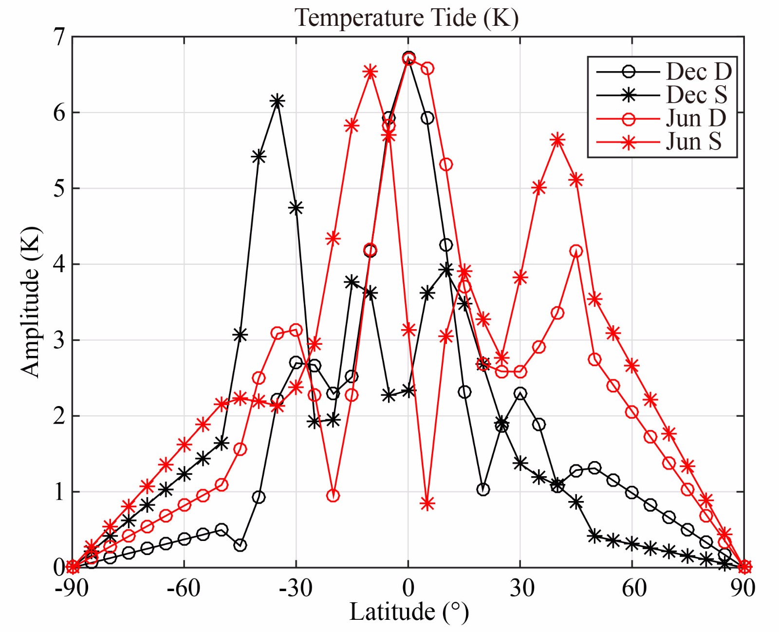
This coupled GCITEM-TIME3D model is used in this investigation. The following simulations (4 cases) are performed at the December Solstice for low (F₁₀₇, F_107A = 70, 2 cases) or high (F₁₀₇, F_107A = 210, 2 cases) solar activity levels, and geomagnetic quiet input with a cross cap potential of 20 kV and auroral particle precipitation with a hemispheric power of 10 GW. An IGRF geomagnetic field is used in these simulations. The GCITEM-TIME3D’s initial and low boundary conditions are derived primarily from MSIS00, HWM93, and IRI 2000 empirical models. However, the low boundary, which is at the height of 90 km, uses the zonal mean states of neutral temperature, neutral density, and neutral compositions from the MSIS00 empirical model and the neutral temperature and density tides from TIMED/SABER observations. These tides include the migrating diurnal tide and the migrating semi-diurnal tide. The details of calculations of these tides from TIMED/SABER observations can be seen in Ren ZP et al. (2011) and Wan W et al. (2012). The low boundary tidal wind is not derived from the input, but from the self-consistent calculation based on the low boundary neutral temperature and neutral density. To analyze the influence of atmospheric tide on the annual anomalies, we use the June Solstice atmospheric tide in some simulations (2 cases) and the December Solstice tide in others (2 cases). Figure 1 shows the latitudinal variations in the amplitude of the December neutral temperature diurnal tide (black cycle line), the December semidiurnal tide (black star line), the June diurnal tide (red cycle line), and the June semidiurnal tide (red star line) at the low boundary of the GCITEM-IGGCAS, in units of K. As shown in Figure 1, an obvious annual asymmetry can be observed in atmospheric tides, and the asymmetry of the semidiurnal tide is stronger than that of the diurnal tide. To keep removing all the effects of the initial conditions, 15 model day runs were made in all simulations to obtain the presented results.

Figure  1.  Latitudinal variations of the amplitude of December neutral temperature diurnal tide (black cycle line), December semidiurnal tide (black star line), June diurnal tide (red cycle line), and June semidiurnal tide (red star line) at the low boundary of the GCITEM-IGGCAS, in units of K.

DownLoad: Full-Size Img PowerPoint

3.   Result and Discussions

Similar to Ren ZP et al. (2014), we focus primarily on the influence of atmospheric tide on the ionospheric zonal mean states, and will analyze mainly the longitudinal and diurnal mean (zonal mean) ionospheric states. The distributions of ionospheric plasma density depend on the geomagnetic field, and the geomagnetic latitude varies with geographic longitude. Thus, we calculate the ionospheric mean states in the quasi-dipole coordinate system (see Richmond, 1995 and Ren ZP et al., 2008 for details).

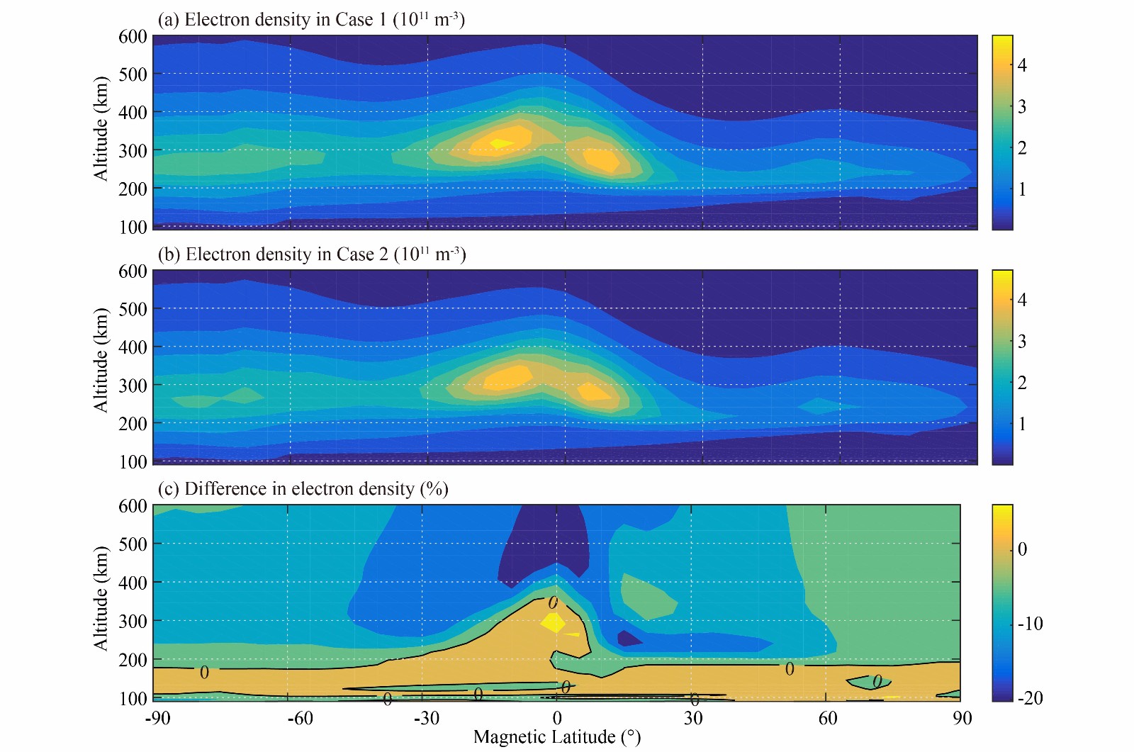
Figure 2a shows latitudinal and altitudinal variations of the zonal mean of the ionospheric electron densities at the December Solstice for low solar activity levels (case 1); Figure 2b shows ionospheric latitudinal and altitudinal variations at the December Solstice driven with the June tide (case 2). We observe that the electron densities in Figures 2a and 2b show similar latitudinal and altitudinal variations, and that their differences are slight. With the ‘fountain effect’, the equatorial ionization anomaly (EIA) appears in the mean electron densities; the low-latitude ionosphere is higher than the mid- and high-latitude ionosphere in both cases. The obvious ionospheric summer–winter (South–North) asymmetries both appear in Figures 2a and 2b, and the electron density in the Southern Hemisphere (summer hemisphere) is significantly higher than that in the Northern Hemisphere (winter hemisphere).

Figure  2.  Altitudinal and latitudinal variations of the simulated zonal mean electron densities, in units of 10¹¹ m^-3, at December, (a) driven by the December atmospheric tide, and (b) driven by the June atmospheric tide. (c) The relative difference (δNe) of the zonal mean electron densities between the two simulations (a) and (b), in units of %.

DownLoad: Full-Size Img PowerPoint

To analyze the effects of tide, we calculated the relative differences between these two cases as follows:

Figure 2c shows the latitudinal and altitudinal variations of δNe in units of %; the solid lines in this figure are the zero lines. Because in these two simulations most of the inputs and boundary conditions are the same, δNe must be driven by the annual asymmetry in the atmospheric tide (that is, by the June–December difference in the atmospheric tide), and must express the influence of atmospheric tide on the annual asymmetry of the zonal mean ionospheric electron density. As shown in Figure 2c, the value of δNe varies mainly between –20% and 10%, and this asymmetry shows obvious latitudinal and altitudinal variations. We first focus on the altitudinal variation of δNe. At lower altitudes (below about 200 km), δNe is mainly larger than zero, and the June tide increases the zonal mean electron density. At higher altitudes (above about 200 km), δNe is mainly less than zero, and the June tide decreases the zonal mean electron density. The obvious summer–winter (South–North) asymmetries can also be found in Figure 2c, and it is suggested that the influence of atmospheric tide shows obvious latitude variation. There is a positive region at the equator and in the low latitudes of the summer hemisphere near the height of 300 km.

To analyse the details, Figure 3 shows the altitudinal profiles of latitudinal mean δNe (black solid line), δNe at –45° (summer middle latitude, black cycle line), δNe at –15° (summer EIA region, black star line), δNe at 0^o (red solid line), δNe at 15° (winter EIA region, red star line), and δNe at 45° (winter middle latitude, red cycle line) in units of %. Although all profiles show similar altitudinal variations in the lower thermosphere region, the altitudinal variations show large differences at higher altitudes. The latitudinal mean δNe profile shows the global mean ionospheric response to atmospheric tide, and its altitudinal variation is more consistent with the profile at middle latitude of the summer hemisphere (Southern Hemisphere). The latitudinal mean δNe profile below 180 km shows weak positive value and above 180 km shows negative value. The negative value increases with altitude between 180 km and 450 km, reaching its maximum near 450 km, and decreases with altitude above 450 km.

Figure  3.  The altitudinal profiles of latitudinal mean δNe (solid line), δNe at –45° (summer middle latitude, dashed line), δNe at –15° (summer EIA region, star line), δNe at 0° (cycle line), δNe at 15° (winter EIA region, plus line), and δNe at 45° (winter middle latitude, cross line) in units of %.

DownLoad: Full-Size Img PowerPoint

In addition to the altitudinal variations, δNe also shows complex latitudinal variations, which vary with altitude. At lower altitude (below 180 km), the latitudinal and altitudinal variations are not significant, and δNe keeps a weak positive value. The ions at low ionosphere are mainly molecular, and the plasma densities are controlled by photochemistry. Hence, the low ionospheric latitudinal variations are mainly controlled by latitudinal variation of the solar zenith angle, and the latitudinal variations of δNe are not significant. However, we observe that there is a small-scale structure at middle latitude of the winter hemisphere (Northern Hemisphere) that may be driven by the vertical propagation of the atmospheric tide. Lindzen (1967) suggested that the diurnal tide can break down in the mesosphere-lower thermosphere (MLT) region, generate turbulence, enhance the eddy mixing, and change the chemical composition in the MLT region and in the higher thermosphere. Because diurnal and semidurunal tides can affect the eddy mixing and change the chemical compositions in MLT region, atmospheric tide can change the NO and O₂ densities in the E-region, and affect the E-region molecular ion (and electron) densities (see Ren ZP et al., 2012b, 2014).

Because ionospheric dynamics play a more important role in the higher than in the lower ionosphere, the altitudinal and latitudinal variations of δNe at the higher ionosphere are more complex than at the lower ionosphere. Moreover, the latitudinal variations at the higher ionosphere are greater than at the lower, and δNe at low-latitudes and at mid- and high-latitudes show different features, which may be driven by different mechanisms. At mid- and high-latitudes, there are obvious latitudinal variations and summer–winter asymmetry (or Southern Hemisphere–Northern Hemisphere asymmetry). At middle latitude of the Southern Hemisphere (summer hemisphere, –45°), the δNe profile (black cycle line in Figure 3) above 180 km shows negative value, which increases with altitude between 180 and 300 km, reaches its maximum near 300 km, and decreases with altitude above 300 km. Above 180 km at middle latitude of the Northern Hemisphere (winter hemisphere, 45°), the δNe profile (red cycle line in Figure 3) also shows negative value, which increases with altitude between 180 and 240 km, reaches its maximum near 240 km, decreases with altitude between 240 and 330 km, and increases with altitude above 330 km. By transporting ions and electrons, the dynamic mechanism can affect the ionospheric electron density, and the wind blowing from the summer hemisphere (Southern Hemisphere) to the winter hemisphere (Northern Hemisphere) may play an important role in the summer–winter asymmetry (or Southern Hemisphere–Northern Hemisphere asymmetry). In addition to dynamic mechanisms, chemical mechanisms may also be important. As mentioned above, atmospheric tide enhances eddy diffusions, can cause enhanced downward transport of atomic oxygen and upward transport of O₂ and N₂, can change the chemical compositions in high thermosphere, and can affect the F-region ionospheric chemical mechanisms.

Different from δNe at mid- and high-latitudes, which are mainly negative, δNe at low-latitudes and the equator appears positive in some regions. At the equator, the δNe profile (red solid line in Figure 3) is positive from 180 to 360 km and negative above 360 km. The positive value increases with altitude between 180 and 290 km, reaches its maximum near 290 km, and decreases with altitude between 290 and 360 km. The negative value increases with altitude between 360 and 520 km, reaches its maximum near 520 km, and decreases with altitude between 520 and 600 km. In the low latitudes of the Northern Hemisphere (winter hemisphere, 15°), the δNe profile (red star line in Figure 3) above 180 km also shows negative values. The negative value increases with altitude between 180 and 240 km, reaches its maximum near 240 km, decreases with altitude between 240 and 370 km, and increases with altitude above 370 km. In the low latitudes of the Southern Hemisphere (summer hemisphere, –15°), the δNe profile (black star line in Figure 3) is positive from 180 to 280 km and negative above 280 km. The positive value increases with altitude between 180 and 220 km, reaches its maximum near 220 km, and decreases with altitude between 220 and 280 km. The negative value increases with altitude between 280 and 380 km, reaches its maximum near 380 km, and decreases with altitude between 380 and 600 km. As shown in Figures 2 and 3, δNe at low-latitudes and the equator mainly appears positive at lower altitude, and appears negative at higher altitude. As shown in Figure 2c, the height of the zero line varies with geomagnetic latitude, and the altitudinal peak of the zero line appears at the magnetic equator. Actually, we can say that EIA appears in δNe, and this structure is driven by the ‘fountain effect’ and upward equatorial vertical E×B plasma drifts. Previous research has suggested that atmospheric tide can affect the ionospheric dynamo, and drive vertical drifts and the ionospheric equatorial ionization anomaly structure (EIA) near the magnetic equator (e.g. Jin et al., 2008; Ren ZP et al., 2009, 2010). Through ionospheric dynamo, the annual asymmetry of atmospheric tide can drive annual asymmetry in the vertical drifts near the magnetic equator, and drive annual asymmetry in the ionospheric EIA.

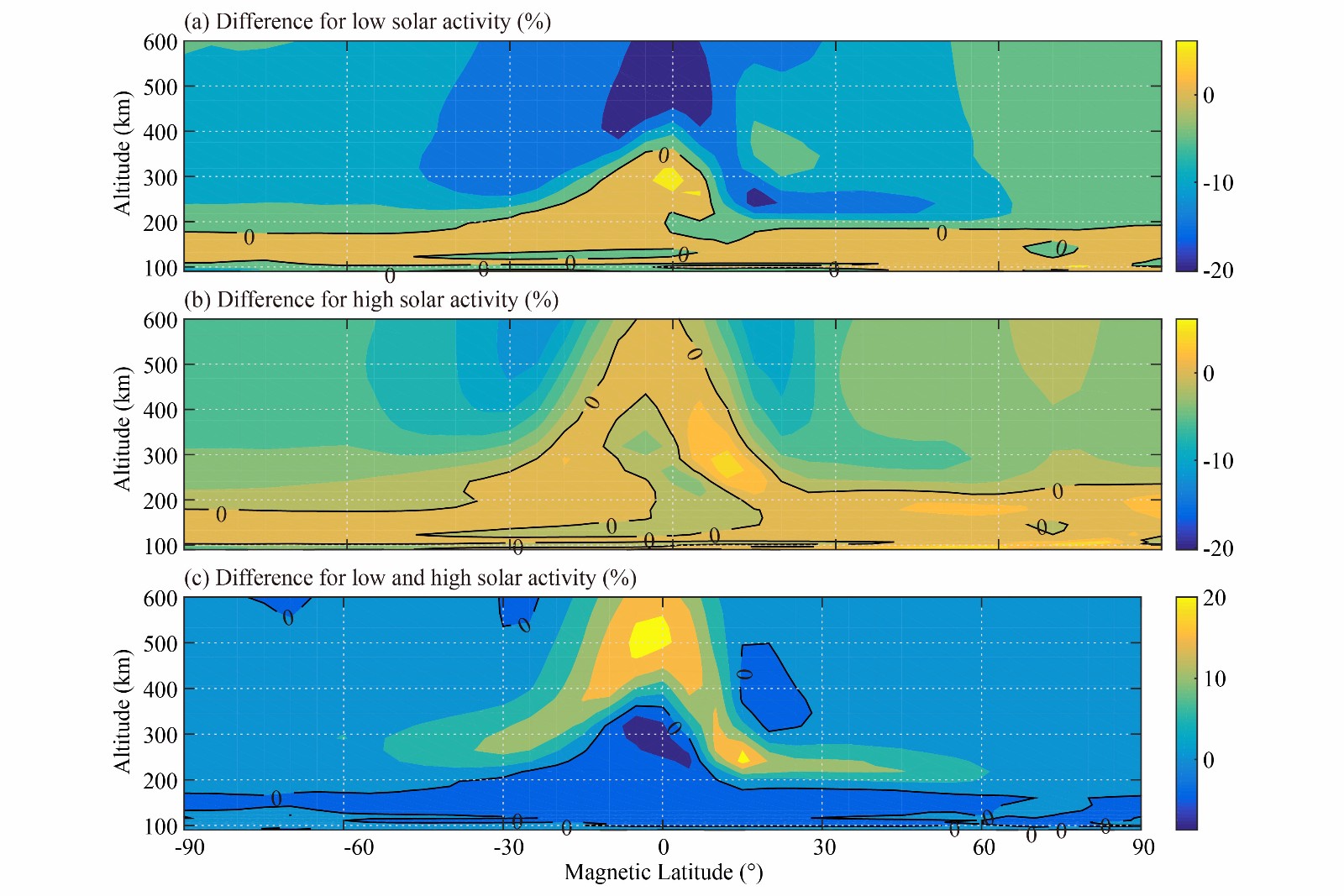
Previous investigations implied that the ionospheric annual anomalies may vary with solar activity level. Hence, we also compare δNe at high solar activity level with that at low solar activity level. Figures 4a and 4b respectively show the latitudinal and altitudinal variations of zonal mean ionospheric electron densities for low solar activity level and for high solar activity level; Figure 4c shows the difference between Figures 4a and 4b. The solid lines in Figures 4a, 4b, and 4c are the zero lines. At the lower ionosphere, the difference between δNe at high solar activity level and at low solar activity level is very slight, and the annual anomaly driven by atmospheric tide does not vary significantly with the increase of solar activity. At higher mid- and high-latitude ionosphere, although δNe at high solar activity levels are mainly smaller than at low solar activity levels, the annual anomaly driven by atmospheric tide mainly decreases with the increase of solar activity. At low-latitude ionosphere, the EIA structure also appears in the δNe at high solar activity level; an EIA-like structure can be found in Figure 4c. Because the equatorial daytime upward drift for high solar flux levels is stronger than for low solar flux levels, the spatial scale of the EIA is larger than that at low solar activity levels.

Figure  4.  The altitudinal and latitudinal variations of the relative difference of the zonal mean electron densities for (a) low solar activity level, for (b) high solar activity level, and (c) for their difference.

DownLoad: Full-Size Img PowerPoint

4.   Summary and Conclusion

The ionospheric annual anomaly is an important ionospheric seasonal variation. Based on the GCITEM-IGGCAS model, we simulated the influence of the annual asymmetry of atmospheric tide on the ionospheric annual anomalies. Through respectively adding June tide and December tide at the model’s low boundary, we find that the tidal influence on the annual anomalies of the ionospheric electron density varies with latitude, altitude, and solar activity level. Compared with the December tide, the June tide mainly increases the ionospheric electron density below the height of 200 km, and mainly decreases the electron density above the height of 200 km. In the low-latitude ionosphere, tide affects the equatorial ionization anomaly structure (EIA) above the height of 200 km, which suggests that tide affects the equatorial vertical E×B plasma drifts. Although below the height of 200 km the tide-driven ionospheric annual anomalies vary insignificantly with the solar flux level, above the height of 200 km the annual anomalies mainly decrease with solar activity.

Acknowledgments

This work is supported by the Strategic Priority Research Program of Chinese Academy of Sciences (Grant No. XDA17010201), the National Natural Science Foundation of China (41674158, 41874179, 41621063, 41427901, 41474133, 41322030), the Youth Innovation Promotion Association CAS (2014057), and the Opening Funding of Chinese Academy of Sciences dedicated for the Chinese Meridian Project.